Graph

Element Graph displays the progression of values in a certain time range (like a line recorder). Example of use are temperatures, counters, power consumption etc.

The telegrams are provided by the ring buffer of the EIBPORT which stores the last 20000 telegrams.

CONTROL L support
This item appears in the CONTROL L. The graph provides some additional functions there in the Java visualization can’t be used. The relevant features are identified in the parameter window with a "*" (asterisk).

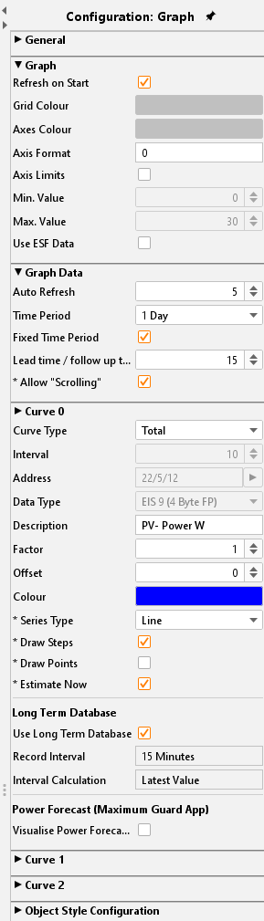
Specific parameters

Please have in mind that the graph elment is only able to display values if it finds any data in the recording table. If the data is a group address as appropriate by a broken clock EIBPORT with a time stamp well before the present, the data will not be shown in the graph (or graph must be scrolled back up to that date)!

Auto Refresh

Once the visualisation is open, the graph updates automatically after this interval (in minutes). Current data from the EIBPORT recording table is retrieved again and new measuring points are calculated.

Time period

Determines the time grid on which the graph is based:

• 1 hours

• 3 hours

• 6 hours

• 12 hours

• 1 days

• 2 days

• 1 weeks

Fixed time period

When activated, the time range will always be displayed from beginning to end. If this option is disabled, the time range will always be back calculated from the present time.

Lead time / follow-up time

Select a time that is slightly greater than the interval between two telegrams on this group address.

This way you make sure that the telegrams just outside the displayed time range are also known, and the line of the graph at the edges of the time range is displayed correctly.

If the time range of your graph regularly starts with a gap before the first telegram value, then the lead time / follow up time is set too small.

Allow „Scrolling" (also available under Java)

This option allows the user to scroll back or forward in the visualization according to the set time range, always assuming that data is available at this point in time.

Calculation

There are two different types possible:

• Total: the value is displayed as absolute value by time. In case of meter readings, the graph would increase continuously.

• Difference: The difference between two values is displayed by time. The frequency between the measurements can be set by „interval“ (Unit = min). The smaller the time gap the more exact the curve will be.

Data type

Several EIS formats are supported:

• EIS 1 (1 Bit)

• EIS 5 (2 Byte FP)

• EIS 6 (1 Byte)

• EIS 9 (4 Byte FP)

• EIS 10s (2 Byte Value)

• EIS 10u (2 Byte unsigned Value)

• EIS 11s (4 Byte Value)

• EIS 11u (4 Byte unsigned Value)

• EIS 14s (1 Byte Value)

• EIS 14u (1 Byte unsigned Value)

• DPT 29 (8 Byte signed Value)

The appendix provides an overview of types of EIS in conjunction with DTP data types.

Description

Enter a legend for the curve. The text is displayed below the graph in the selected colour curve.

Factor / Offset

Using factor and offset, the input value to be formatted as desired. The value is multiplied by a factor and added to the offset.

Colour

Defines the colour of the curve and the labelling.

Curve type

(only possible for CONTROL L) The curve type determines which diagram form is displayed. The following can be selected:

• Line: A line diagram is drawn.

• Area: An area diagram is created in which the area below the line is marked accordingly.

Draw Steps

(only possible for CONTROL L) Prevents the linear connection of successive telegram values. This way you get a more sensible representation as a square wave e.g., for EIS1 values.

Draw Points

(only possible for CONTROL L) The individual measuring points are marked on the line of the graph when activated.

Estimate Now

(only possible for CONTROL L) – only possible if "Draw steps" is enabled. This extends the line of the graph after the last telegram. In the current time period, it will be extended to the current time, in past time periods it will be extended to the end of the respective time period.

This option thus "hides" at least at the end of the time range a possibly too small lead time / follow up time.

If the time range of your graph regularly starts with a gap before the first telegram value even after activating this option, then the lead time / follow up time is too small.

Activate long-term recording / recording

Activating the recording opens the dialog to the long-term database. After selecting or creating a database (as described in chapter 5.2.1.3 EXTRAS / long-term databases) the data will be:

• Recording interval

• Interval calculation

transferred to the configuration menu. Because of that, these data are available in the graph element to display. Depending on the visualization, whether within JAVA or as WEB browser, e.g., CONTROL L, the selection of display is different.

Object style configuration

All other options are described in chapter General Element Parameter.

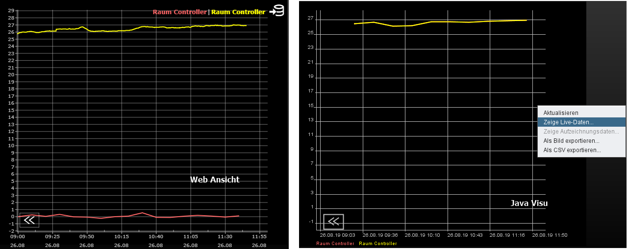
Functionality within the visualization

Within the visualization the element provides some more functions. These functions can becalled by right-button mouse click.

• update: updates the value.

• Show live data: Change to display the live data.

• Show recording data: Change to the display of the long-term data.

• Export as graphic…: Opens the file browser for saving the graph as file (*.png).

• Export as CSV…: Opens the file browser for saving the graph as csv file

Control L functionality within the visualisation

In contrast to the graph in the Java Visualisation has the graph at CONTROL L a zoom function and curve information.

For switching between the live data and the data of the long-term recording, an icon (top right) appears, which is to be clicked on.

Zoom Function

The mouse is inside the graph element can be in and zoomed out again with the mouse wheel in the graph. Can also hold down the mouse button to select one area to be marked on the graph, which is then enlarged. With a double click anywhere in the field of graph unmagnified view is restored.

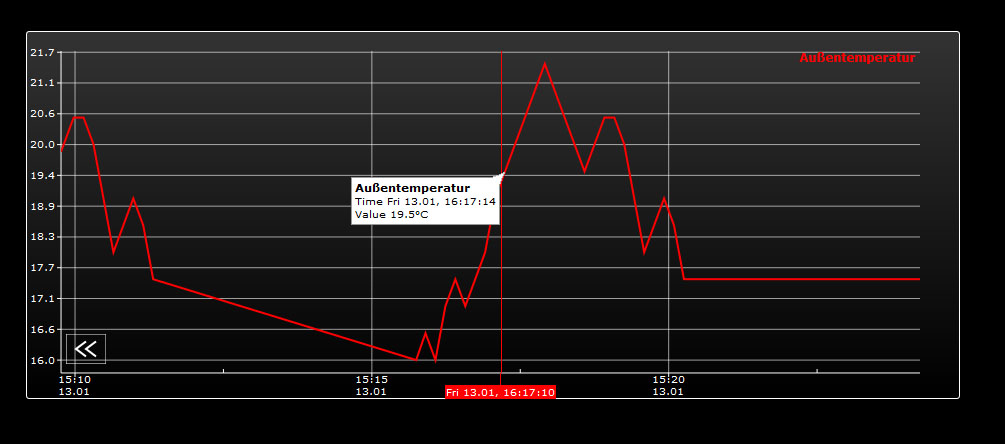
Curve information

If you use the mouse pointer moves along the curve recording, useful information related to the measurement point are shown curve name, time / date and the measured value.

Information about the recording table (ringbuffer)

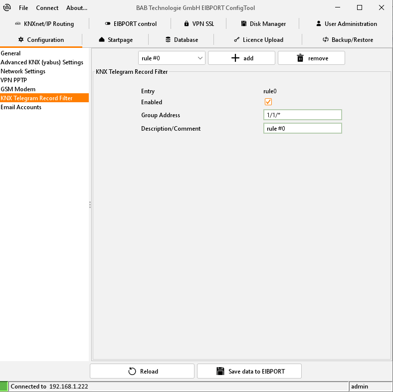
The Graph element uses values from the past, so it has to access data from the ring buffer of the EIBPORT (EIB recording table). This buffer contains about 500.000 telegrams. The eldest telegram is replaced by the latest one. Within a KNX/EIB installation 500.000 telegrams possibly may be transmitted within some hours. So, the Graph is provided just with data from this time range. In this case the recording filter serves as remedy.

If the Graph should be enabled to display if consumption data for a longer time range the recording filter has to be used. This filter defines the group address(es) which should be stored in the buffer.

The filter can be called and rules can be defined under „System“ > „Configuration“ > „EIB Recording filter“. Either group addresses or group address ranges can be selected. In case of address ranges a wildcard (*) should be used:

Example:
“1/*/*” (without quotation mark) means that just data from the main line “1” will be buffered. If the filter is set to “1/1/*” the middle group is filtered. Alternatively, the wanted address is typed in.